CNN在计算机视觉领域取得了很好的结果,同时它可以应用在文本分类上面,此文主要介绍如何使用tensorflow实现此任务。
CNN实现文本分类的原理
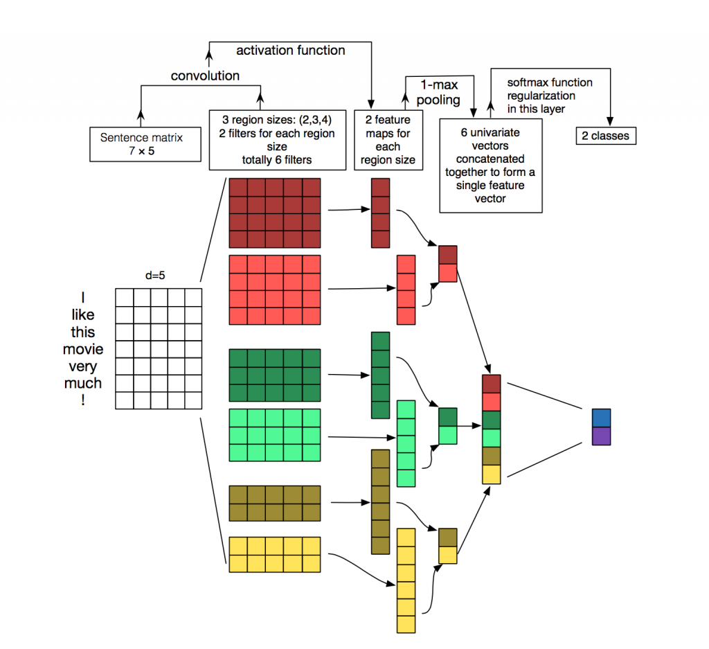
下图展示了如何使用cnn进行句子分类。输入是一个句子,为了使其可以进行卷积,首先需要将其转化为向量表示,通常使用word2vec实现。d=5表示每个词转化为5维的向量,矩阵的形状是[sentence_length ×× 5],即[7 ×× 5]。6个filter(卷积核),与图像中使用的卷积核不同的是,nlp使用的卷积核的宽与句子矩阵的宽相同,只是长度不同。这里有(2,3,4)三种size,每种size有两个filter,一共有6个filter。然后开始卷积,从图中可以看出,stride是1,因为对于高是4的filter,最后生成4维的向量,(7-4)/1+1=4。对于高是3的filter,最后生成5维的向量,(7-3)/1+1=5。卷积之后,我们得到句子的特征,使用activation function和1-max-pooling得到最后的值,每个filter最后得到两个特征。将所有特征合并后,使用softmax进行分类。图中没有用到chanel,下文的实验将会使用两个通道,static和non-static,有相关的具体解释。
这里写图片描述
本文使用的模型
这里写图片描述
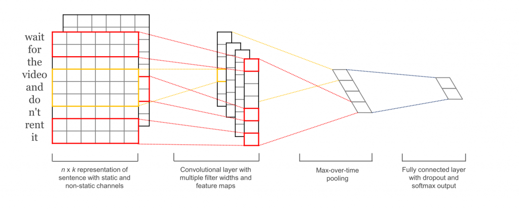
主要包括五层,第一层是embedding layer,第二层是convolutional layer,第三层是max-pooling layer,第四层是fully connected layer,最后一层是softmax layer.接下来依次介绍相关代码实现。
1 2 3 4
| # Placeholders for input, output and dropout self.input_x = tf.placeholder(tf.int32, [None, sequence_length], name="input_x") self.input_y = tf.placeholder(tf.float32, [None, num_classes], name="input_y") self.dropout_keep_prob = tf.placeholder(tf.float32, name="dropout_keep_prob")
|
tf.placeholder 创建一个占位符变量,在训练或者测试的时候,需要将占位符输入到网络中进行计算,其中的第二个参数是输入张量的形状。None 意味着它可以是任何维度的长度,在我们的实验中它代表批处理的大小,None使得网络可以处理任意长度的batches。
失活率同样也是输入的一部分,在训练的时候使用dropout ,测试的时候不使用dropout 。
EMBEDDING LAYER
这一层将单词索引映射到低维的向量表示,它本质上是一个查找表,我们从数据中通过学习得到。
1 2 3 4
| with tf.device('/cpu:0'), tf.name_scope("embedding"): W = tf.Variable(tf.random_uniform([vocab_size, embedding_size], -1.0, 1.0), name="W") self.embedded_chars = tf.nn.embedding_lookup(W, self.input_x) self.embedded_chars_expanded = tf.expand_dims(self.embedded_chars, -1)
|
其中,W 是 在训练时得到的embedding matrix.,用随机均匀分布进行初始化。tf.nn.embedding_lookup实现embedding操作,得到 一个3-dimensional 的张量,形状是 [None, sequence_length, embedding_size]. sequence_length 是数据集中最长句子的长度,其他句子都通过添加“PAD”补充到这个长度。embedding_size 是词向量的大小。
TensorFlow的卷积函数-conv2d 需要四个参数, 分别是batch, width, height 以及channel。 embedding之后不包括 channel, 所以我们人为地添加上它,并设置为1。现在就是[None, sequence_length, embedding_size, 1]
CONVOLUTION AND MAX-POOLING LAYERS
由图中可知, 我们有不同size的filters。因为每次卷积都会产生不同形状的张量,所以我们要遍历每个filter,然后将结果合并成一个大的特征向量。
1 2 3 4 5 6 7 8 9 10 11 12 13 14 15 16 17 18 19 20 21 22 23 24 25 26 27 28
| pooled_outputs = [] for i, filter_size in enumerate(filter_sizes): with tf.name_scope("conv-maxpool-%s" % filter_size): # Convolution Layer filter_shape = [filter_size, embedding_size, 1, num_filters] W = tf.Variable(tf.truncated_normal(filter_shape, stddev=0.1), name="W") b = tf.Variable(tf.constant(0.1, shape=[num_filters]), name="b") conv = tf.nn.conv2d( self.embedded_chars_expanded, W, strides=[1, 1, 1, 1], padding="VALID", name="conv") # Apply nonlinearity h = tf.nn.relu(tf.nn.bias_add(conv, b), name="relu") # Max-pooling over the outputs pooled = tf.nn.max_pool( h, ksize=[1, sequence_length - filter_size + 1, 1, 1], strides=[1, 1, 1, 1], padding='VALID', name="pool") pooled_outputs.append(pooled) # Combine all the pooled features num_filters_total = num_filters * len(filter_sizes) self.h_pool = tf.concat(3, pooled_outputs) self.h_pool_flat = tf.reshape(self.h_pool, [-1, num_filters_total])
|
这里W 是filter 矩阵,h 是对卷积结果进行非线性转换之后的结果。每个 filter都从整个embedding划过,不同之处在于覆盖多少单词。 “VALID” padding意味着没有对句子的边缘进行padding,也就是用了narrow convolution,输出的形状是 [1, sequence_length - filter_size + 1, 1, 1]。narrow convolution与 wide convolution的区别是是否对边缘进行填充。
这里写图片描述
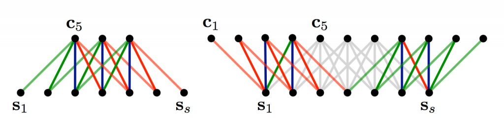
Narrow vs. Wide Convolution. Filter size 5, input size 7. Source: A Convolutional Neural Network for Modelling Sentences (2014)
当你的filter比输入的size还大时,你可以看到wide convolution是多么的有用,甚至说是必须的。如上所示,narrow convolution产出的尺寸是(7-5)+1=3,而wide convolution产出尺寸是(7+2*4-5)+1=11。通常,输出尺寸的规则表达式为:
这里写图片描述
对输出进行max-pooling后得到形状是 [batch_size, 1, 1, num_filters] 的张量,本质上是一个特征向量,最后一个维度是特征代表数量。把每一个max-pooling之后的张量合并起来之后得到一个长向量 [batch_size, num_filters_total]. in tf.reshape 中的 -1表示T将向量展平。
DROPOUT LAYER
Dropout也许是cnn中最流行的正则化方法。dropout的想法很简单,dropout layer随机地选择一些神经元,使其失活。这样可以阻止co-adapting,迫使它们每一个都学习到有用的特征。失活的神经单元个数由dropout_keep_prob 决定。在训练的时候设为 0.5 ,测试的时候设为 1 (disable dropout) .
1 2 3
| # Add dropout with tf.name_scope("dropout"): self.h_drop = tf.nn.dropout(self.h_pool_flat, self.dropout_keep_prob)
|
SCORES AND PREDICTIONS
利用特征向量,我们可以用矩阵相乘计算两类的得分,也可以用 softmax函数计算两类的概率值。
1 2 3 4 5
| with tf.name_scope("output"): W = tf.Variable(tf.truncated_normal([num_filters_total, num_classes], stddev=0.1), name="W") b = tf.Variable(tf.constant(0.1, shape=[num_classes]), name="b") self.scores = tf.nn.xw_plus_b(self.h_drop, W, b, name="scores") self.predictions = tf.argmax(self.scores, 1, name="predictions")
|
LOSS AND ACCURACY
可以用得分定义损失值。损失计算的是网络的误差,我们的目标是将其最小化,分类问题标准的损失函数是交叉熵损失。
1 2 3 4
| # Calculate mean cross-entropy loss with tf.name_scope("loss"): losses = tf.nn.softmax_cross_entropy_with_logits(self.scores, self.input_y) self.loss = tf.reduce_mean(losses)
|
计算正确率
1 2 3 4
| # Calculate Accuracy with tf.name_scope("accuracy"): correct_predictions = tf.equal(self.predictions, tf.argmax(self.input_y, 1)) self.accuracy = tf.reduce_mean(tf.cast(correct_predictions, "float"), name="accuracy")
|
MINIMIZING THE LOSS
利用TensorFlow 内置的optimizers,例如 Adam optimizer,优化网络损失。
1 2 3 4
| global_step = tf.Variable(0, name="global_step", trainable=False) optimizer = tf.train.AdamOptimizer(1e-4) grads_and_vars = optimizer.compute_gradients(cnn.loss) train_op = optimizer.apply_gradients(grads_and_vars, global_step=global_step)
|
train_op 是一个新建的操作,我们可以在参数上进行梯度更新。每执行一次 train_op 就是一次训练步骤。 TensorFlow 可以自动地计算才那些变量是“可训练的”然后计算他们的梯度。通过global_step这个变量可以计算训练的步数,每训练一次自动加一。
CHECKPOINTING
TensorFlow 中可以用checkpointing 保存模型的参数。checkpointing中的参数也可以用来继续训练。
1 2 3 4 5 6 7
| # Checkpointing checkpoint_dir = os.path.abspath(os.path.join(out_dir, "checkpoints")) checkpoint_prefix = os.path.join(checkpoint_dir, "model") # Tensorflow assumes this directory already exists so we need to create it if not os.path.exists(checkpoint_dir): os.makedirs(checkpoint_dir) saver = tf.train.Saver(tf.all_variables())
|
DEFINING A SINGLE TRAINING STEP
用一个batch的数据进行一次训练。
1 2 3 4 5 6 7 8 9 10 11 12 13 14 15
| def train_step(x_batch, y_batch): """ A single training step """ feed_dict = { cnn.input_x: x_batch, cnn.input_y: y_batch, cnn.dropout_keep_prob: FLAGS.dropout_keep_prob } _, step, summaries, loss, accuracy = sess.run( [train_op, global_step, train_summary_op, cnn.loss, cnn.accuracy], feed_dict) time_str = datetime.datetime.now().isoformat() print("{}: step {}, loss {:g}, acc {:g}".format(time_str, step, loss, accuracy)) train_summary_writer.add_summary(summaries, step)
|
train_op 什么也不返回,只是更新网络中的参数。最终,打印出当前训练的损失值与正确率。如果batch的size很小的话,这两者在不同的batch中差别很大。因为使用了dropout,训练的metrics可能要比测试的metrics糟糕。
同样的函数也可以用在测试时。
1 2 3 4 5 6 7 8 9 10 11 12 13 14 15 16
| def dev_step(x_batch, y_batch, writer=None): """ Evaluates model on a dev set """ feed_dict = { cnn.input_x: x_batch, cnn.input_y: y_batch, cnn.dropout_keep_prob: 1.0 } step, summaries, loss, accuracy = sess.run( [global_step, dev_summary_op, cnn.loss, cnn.accuracy], feed_dict) time_str = datetime.datetime.now().isoformat() print("{}: step {}, loss {:g}, acc {:g}".format(time_str, step, loss, accuracy)) if writer: writer.add_summary(summaries, step)
|
TRAINING LOOP
通过迭代数据进行训练。
1 2 3 4 5 6 7 8 9 10 11 12 13 14 15
| # Generate batches batches = data_helpers.batch_iter( zip(x_train, y_train), FLAGS.batch_size, FLAGS.num_epochs) # Training loop. For each batch... for batch in batches: x_batch, y_batch = zip(*batch) train_step(x_batch, y_batch) current_step = tf.train.global_step(sess, global_step) if current_step % FLAGS.evaluate_every == 0: print("\nEvaluation:") dev_step(x_dev, y_dev, writer=dev_summary_writer) print("") if current_step % FLAGS.checkpoint_every == 0: path = saver.save(sess, checkpoint_prefix, global_step=current_step) print("Saved model checkpoint to {}\n".format(path))
|
VISUALIZING RESULTS IN TENSORBOARD
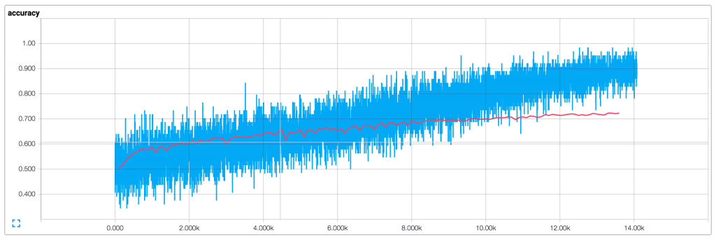
这里写图片描述
这里写图片描述
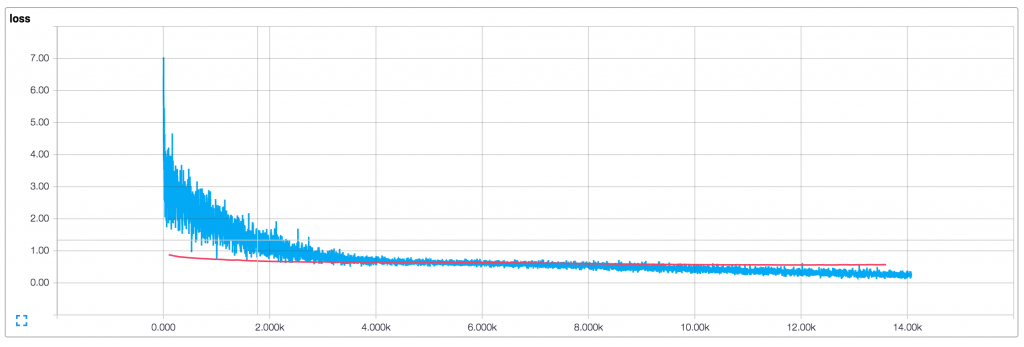
从上图中我们可以观察到:
- 我们的训练 metrics不平滑,因为用的batch sizes很小。如果用大的batches (或者在整个测试集上进行评估),会得到平滑的线。
- 测试集的 accuracy明显比训练集的低,说明网络过拟合了,我们应该用更大的数据集,更强的正则化,更少的模型参数。
- 训练集上的 loss 和 accuracy比测试集低的原因是用了dropout.